I’ve spent the last 6 months working on Spall, trying to push the limit on bigger and bigger traces, and slashing load-times to make that possible. My pie in the sky ideal is to load a 1 TB trace in a human-friendly amount of time, and display it at 60+ fps.
With the current auto-tracing format, every function eats 32 bytes, so that’d be somewhere around 32 billion events in a trace file. The maximum dump rate from the auto-tracer is around 45 million events per second per core, limited mostly by the users’s clockspeed, RDTSC implementation, and linear disk write speed.
Doing a little napkin math, 45M/s is about ~1.5 GB/s of data, so assuming it takes as long to load a file as it does to trace it, it would take ~11 minutes to generate, and another 11 minutes to load that trace. Unfortunately, we’re not quite there yet. I’ve recently made some big performance improvements to get closer to that ideal though! The old build of Spall-native manages somewhere around ~350 MB/s, the new changes I’ve made bring it to around ~650 MB/s, end-to-end.
One of the important things Spall does to render big traces quickly is the LOD (level-of-detail) tree. Spall takes the trace timeline and divides it into slices that can be searched quickly, so rather than scanning gigabytes of data per frame, it can dig into to the big array of functions with only a few lookups, getting functions on screen way faster.
So, what changed to make larger traces faster and lighter to load? I did a big revamp of the LOD building system. The old system used an explicit 4-ary tree, splitting the timeline into quarters, with 4 functions per tree-leaf.
The old tree had indexes in each node to help find its children, and every leaf contained an index into the function array, along with a flag to indicate that the node was a leaf. It ate about ~5 GB per 12 GB trace, all on its own.
Old Explicit Tree Layout
ChunkNode :: struct #packed {
	start_time:       i64,
	end_time:         i64,

	avg_color:      FVec3,
	weight:           i64,

	tree_start_idx:  uint,
	event_start_idx: uint,

	tree_child_count:  i8,
	event_arr_len:     i8,
}
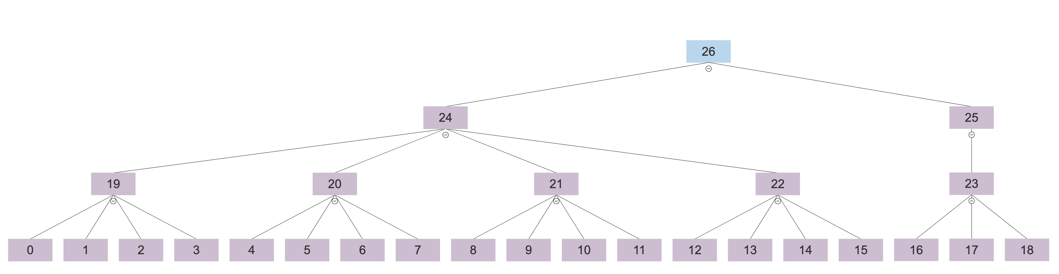
The new LOD is way more space efficient! I’ve moved to an implicit tree, with 32 functions per tree-leaf. The tree is now an eyztinger tree, so we don’t need to store indexes for functions and tree nodes, they can now be computed on the fly. The new setup uses about 5% of the trace size in LOD memory, so an 11 GB trace across 64 threads from GDB eats about ~550 MB of RAM for the LOD structure instead of ~5 GB.
New Implicit Tree Layout
ChunkNode :: struct #packed {
	start_time:  i64,
	end_time:    i64,

	avg_color: FVec3,
	weight:      i64,
}
For more on Eytzinger Trees, Algorithmica has a solid overview.
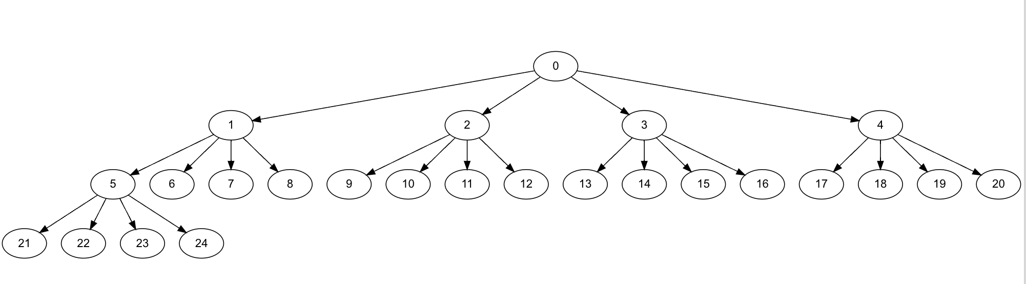
The big win here is that the index of the left child of a node is kn + 1, where k is the arity of the tree,
(binary, ternary, 4-ary, etc.), and n is the current node’s index.
So, for node 5, the left child is 4*5+1 or 21, and none of that information needs to be stored.
This along with an increase in the number of functions per leaf, did come at the cost of framerate, although with recent render-performance improvements, I had enough frame-budget to dial back RAM a bit more. Now, on my older Intel Mac, rather than running at 200 frames per second, I only get 60 fps for large (6 GB+) traces, and on beefier machines, I’m down from 400 fps to 200. What a tragedy! :P
I figure, if we’ve got the headroom, might as well use it for something worthwhile. There’s still plenty of performance improvements left on the table to make. I haven’t started working with threads yet, although I’ve been designing the ingest pipeline and renderer with threads in mind. I should be able to parallelize both rendering and loading files, which’ll give us a nice little boost because the trace data has few cross-thread dependencies, so it can be split across a work-pool without too much effort.